Between 2005 and 2008, I worked on various instrument control modules within Thermo Fisher Scientific’s Atlas desktop chromatography data system (CDS).
Chromatography and Instruments
Wikipedia has a good set of articles on the subject of chromatography, but basically it is a type of separation analysis: that is, we can quantify the individual components of a substance by breaking it apart through some linear process that affects each component differently. With a little bit of experimentation, the basic technique can be demonstrated with household materials such as coffee filters, magic markers, and water or alcohol (depending on the type of markers used). However, in the lab more precision is needed and hence equipment costing tens of thousands of dollars.
At Themo I worked with a number of different gas- and liquid-chromatography (GC and LC) instruments, but primarily focused on Agilent’s 1100 (and later 1200) LC series, which is pictured here.
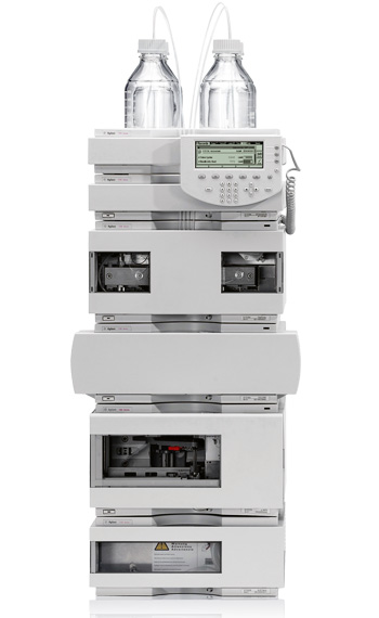
- a pump for pushing solvents through the system (a single solvent, or a blend of solvents)
- some kind of injector to get samples into the stream (often as part of an autosampler unit that can hold dozens of samples at a time)
- a separation column, usually inside of a temperature-controlled unit
- one or more detectors to measure some aspect of the components as they come out of the column (such as how much light of certain wavelengths is absorbed or emitted)
Many high-performance LC (HPLC) instruments from various manufacturers allow for these subcomponents to be reconfigured to a degree, but most often the main instrument is in a single housing and only certain parts can be swapped. Agilent’s 1100/1200 series, on the other hand, was designed for modularity from the start. Each module is in its own housing and selected modules are stacked on one another and plumbed together to form a complete system. There’s also a data connection between the modules and typically a handheld controller.
This modularity even applied down to sub-components such as the network connection, which at the time was an optional plug-in board. This was a problem for me when I first started on the project, because the instrument I was attempting to use didn’t actually have a network card. One obvious choice was to order a new one from Agilent, at a cost of several hundred dollars and some lost days of time. But we had another potential option, owing to the fact that Agilent had been spun off from Hewlett-Packard’s medical and instruments division in the late 1990s: all we really needed was a plain ol’ JetDirect card from an HP laser printer! Sadly, no-one in the office wanted to sacrifice their printing capabilities for the greater good, but with a little help from the internet, I tracked down an available card from a second-hand computer parts dealer about half an hour away and picked it up for about 25 bucks plus train fare.
Atlas Architecture
I never delved into the full development history of Atlas, but I know that it had evolved from at least one older VAX product and seemed to have had a number of different layers wrapped around it over the years, each with its own protocols and conventions. The main user application was written in C++ using Microsoft’s Foundation Class (MFC) library and its document/view framework, but persistence was handled with a third-party table library that basically mapped plain-ol’ C structures in and out of memory (no indexing or strong relationships between tables, as far as I recall). Instruments from different vendors were supported through a plugin-type architecture, and the instrument controllers were typically released on a different schedule from the main product.
Each instrument controller itself consisted of three main components:
- The actual device controller, an out-of-process COM server responsible for communications with the instrument
- A status plugin, an in-process COM server that communicated with the device controller and allowed the user to view the instrument’s current status as well as some direct control of the instrument
- An instrument and method editor DLL (not using COM) that hosted dialogues and associated classes for the user to edit instrument configuration and acquisition method properties
Typically the device controller component would run on a dedicated data server, which could support up to four separate instruments, but it was also possible to run the entire system on a stand-alone workstation. Communication between components for command-and-control actions was generally through COM, but batch submission of jobs from the main application to the device controller and buffering of the acquired data were handled through the file system.
The first version of the 1100 instrument controller that I worked on was nominally 2.0, but part of the code was based on an older driver that had used GPIB for communications rather than a LAN interface. That didn’t concern me so much as I wasn’t working at the communications level at this point, but as in the main application, it did mean that I had to deal with large sections of code with a long history.
Diode Array Detector Support
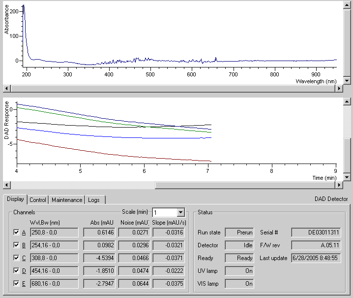
The main focus for this release was full support for the 1100 series diode array detector (DAD). This kind of detector measures light absorbance, and operates within a range of wavelengths in the UV and visible spectrum. The DAD uses an array of photo-sensitive elements to sense the whole spectrum at once, but usually only certain wavelengths are actually of interest, depending on the particular substance being analysed. Thus, the instrument can be configured to electronically filter out the desired bands from the spectrum into discrete channels. Version 1.0 of the control supported only a single wavelength channel, although the target wavelength could be changed during an analysis, making operation very similar to a variable wave detector (VWD), a related, but simpler instrument.
I extended the control to support up to five discrete wavelength channels plus the spectral channel itself. This mainly involved changing the UI to include extra controls, rejigging certain variables to be arrays or lists instead of single members, and wrapping loops around certain parts of the code.
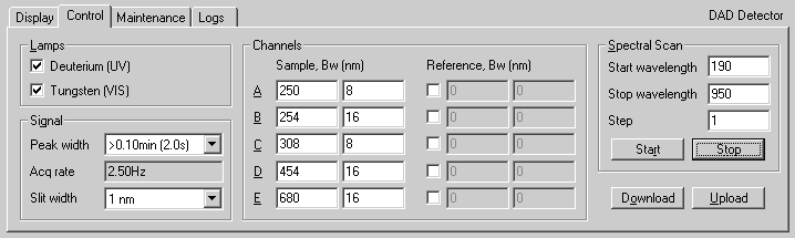
This release also added support for direct control of some basic functions of the DAD from within the status plugin. Notably, users could turn the detector’s lamps on or off, change the acquisition frequency of all the channels, change the spectral range, and perform diagnostic tests. Direct control of an instrument was allowed only when a sample run was not in progress of course, and was principally intended for instrument preparation before a run. Thus, the user could start warming up the instrument and monitor its stability visually from their desktop before starting a run.
Wellplate Autosamplers and Additional Module Versions
The primary feature introduced in the next version of the controller was support for Agilent’s new wellplate autosampler modules. In Agilent’s standard autosampler, all samples are held in closed vials (typically 2ml) and the vials are held in a tray. When a sample needs to be injected into the system, a gripper arm moves to the specified position within the tray, picks up the vial, and moves it over to the syringe for drawing. In a wellplate autosampler, however, the samples are held in an array of open wells, and it is the needle itself that moves over to the specified sample for drawing. A wellplate autosampler can also be used with vials by changing the tray type.
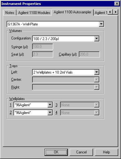
These differences affect the way sample positions are specified between the two models (sequential vial number or row, column notation) and hence some fairly complicated data validations, but in a couple of cases, we needed to skip validations entirely. The first case arose because it was possible to upgrade the instrument driver without actually reconfiguring existing instruments, hence the additional configuration settings would be missing. In this case, we wanted to preserve existing behaviour exactly and didn’t validate the vial ID at all. (Invalid values would eventually be caught and reported by the instrument when the autosampler command was sent.) The second case arose by design because the tray geometry was configured as part of instrument settings rather than method settings, and had a higher security level; in some labs only administrators were permitted to change the instrument configuration but analysts were not. Eventually I would have planned to add an administrator option to allow the tray configuration to be specified in the method, but for the meantime, we simply allowed the administrator to leave the tray configuration empty. For this case, in the sequence editor we validated only that the vial ID was in the correct format (either a single number, or a four-part position), but not the actual ranges.
Enhanced Instrument Control and Reporting
The next and last major version of the controller that I worked on (aside from a couple of subsequent patch releases) was quite the most interesting and satisfying one for me. In addition to a number of miscellaneous new features, this version focused broadly on two major areas: enhanced direct instrument control and reporting in the status plugin, and support for the new 1200 series of modules that were just coming out.
The latter issue was the highest priority, since any new instruments that customers might purchase would be from the 1200 series, and we did not know initially whether the existing controller would support them. The 1200 series modules could be configured with special firmware for them to operate in compatibility mode with the 1100 series, but we needed to run tests to make sure. Beyond that, when running in native mode, there was a new data format for the detectors and some minor changes in control commands.
In terms of direct instrument control, while we had added a lot of control for the DAD in version 2 of the status plugin, we hadn’t really done anything with the other modules, and over the years a number of requests from customers had accumulated for additional parameters across the whole stack. For example, they wanted to be able to control the lamps for other detectors, turn the pump on and off and change the solvent composition and flow rate, and control the heater temperature. There were also a couple of requests to slightly change the arrangement and format of current control commands for the DAD. For example, the lamp on/off control was implemented as a checkbox, but since this actually resulted in an operation on the instrument, it seemed that [On] and [Off] buttons would be clearer.
There was also a need to improve the detail of the status messages coming back from the instrument. All modules in the system had what were called ready/not ready states, indicating whether or not the module was ready to start an analysis. Some of these were transient (eg, heater warming up to setpoint) and some could potentially be fixed directly from the plugin (eg, detector lamps off). However many conditions required physical action at the instrument (eg, pump out of solvents, autosampler door open), and the main problem was that the plugin didn’t distinguish between the various states: a module was either simply ready or not ready and so virtually all problems required the analyst to walk over and check the instrument regardless. (This was especially difficult for me when I was trying to control one of our instruments in the U.K. from our office in Philadelphia.)
Overall, these requirements represented a significant number of user interface changes, but there weren’t any grand ideas about implementing them, other than simply adding the appropriate controls to each of the existing panels. My gut feeling, however, was that this was going to be increasingly cumbersome. The existing plugin design had one page for each detector type, and one page for all of the other modules on the stack (pump, heater, autosampler, etc). Most of the detector pages were quite simple, but the DAD page had four tabs of its own, with all of the controls that I had added for version 2. Simply expanding this pattern seemed like it would result in an awkward visual layout and would require lots of switching between tabs by users, and on that basis alone I wanted to bring some better organisation to the plugin.
At the same time, I had learned enough about chromatography and our customers that I thought perhaps that these requirements as listed didn’t go far enough. As well as the six or eight setpoints and functions that had been specifically requested, I knew that there were many others that could be helpful to have available from the desktop. Also, while we were plotting detector output over time in the plugin, we weren’t plotting any of the actual values from other modules such as heater temperature or pump pressure. Being able to monitor those over time seemed like it would be useful.
After discussing these ideas briefly with my product managers, I was given a lot of latitude to design things as I saw fit. I made two major structural changes to the user interface of the status plugin, which allowed all of the other elements to fall neatly into place.
First, rather than having one tab for the non-detector modules and a separate tab for each detector, I combined all of the modules on a single tab, where each module was in its own collapsible pane with an additional pane representing the entire system. The system pane contained all the buttons for turning on individual modules rather than having these within each module’s pane and it started out in the expanded state rather than collapsed. The header bar for each module section toggled the visibility of the pane and indicated the module’s ready/not ready state by colour and icon. The idea behind this was that at the start of the day, the analyst could simply open the plugin, start everything warming up in one place, and then attend to the individual module details only as needed.
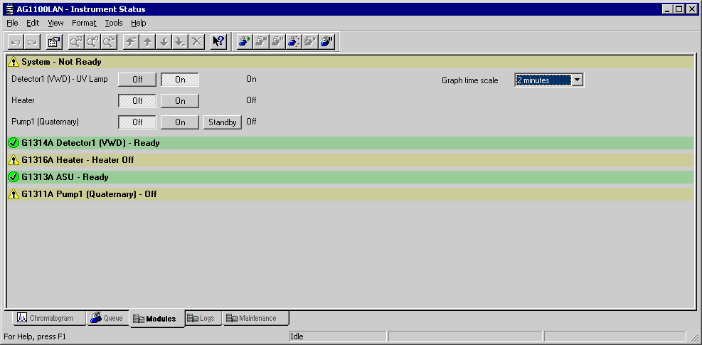
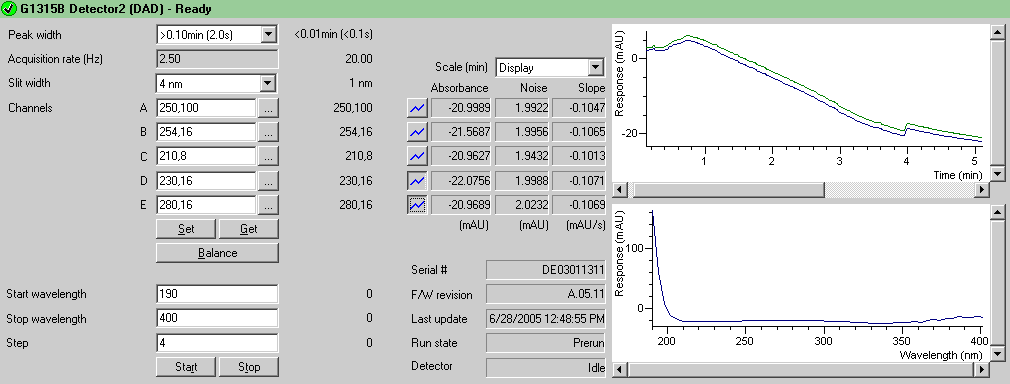
The second major change was that rather than having separate tabs for the display and control of setpoints, I arranged these as two separate columns within each pane, with a common label to the left. Module info and statistics, where applicable, were grouped in an another column, and graphs were shrunk down and moved all the way to the right. The columns were aligned across all modules. Thus, the DAD pane below encompasses all of the functionality of the two tabs shown previously for version 2.0, except for the lamp buttons.
This left the Logs and Maintenance tabs from the DAD. I changed these to being tabs within the overall plugin, and then used the same collapsible pane design for each of the modules within the tabs. This allowed us to more easily extend these features to the rest of the modules. (Logging is virtually identical for each module, so this was enabled almost at a stroke, but we did not develop maintenance features for the other modules because they are highly specialised.)
In addition to the user interface, I also reworked large parts of the internal architecture that were strained by the new requirements. For example, all of the existing control commands and status updates between the plugin and device controller were handled as separate messages, but with a slew of new parameters that was going to be rather chatty. So I combined all of the parameters that naturally went together for each module into a single message for each.
Also due to the existing design, the system could not handle dynamic configuration changes on the stack very well. Whenever communication with the instrument was established, there was a process of matching what the user had manually configured against what the instrument itself was reporting. This process was driven from the stored configuration side rather than the instrument side, so it was not able to handle change events reported by the communications layer very well. In code, each module was represented by its own top-level class, and the instrument-wide container class had a separate member for each possible module that could be configured. I changed this to have a base class for all modules and specialisations for each, with a dynamic list of modules held in the instrument container. Thus, every time the communications library reported a change, the list could be modified dynamically.
I also changed the command messages between the device controller and the plugin to be keyed by a bitmapped value rather than by name. Based on fields in the bitmap, it was then easy to determine whether a particular command was for a specific module or for all modules and despatch accordingly. With these new structures in place, I was able to reduce many long sequences of previously copied-and-pasted if…endif and switch…case with simple loops and virtual functions.
Large rewrites are never without risk, and there were a few minor issues that arose from these changes. There were also a couple of unforeseen effects from other new features as they had been designed. For example, one feature not mentioned above that we had added was logging of instrument actual values at periodic intervals during a run, but this wound up adding many megabytes of data to each workbook file, and so we had to add an option to lengthen the interval or turn it off. However, we patched these issues quickly and all-in-all the radically new design was welcomed enthusiastically.
The Road Not Taken
After these patch releases, I started working on ideas for the next version of the control on my own for a while. I was already aware of some new features that had been requested by customers, some of which required deeper level changes to the communications library. Also, over the years, I had had many chats with the product managers about things they had wanted but weren’t sure were possible or practical. For example, many customers had been asking for automatic instrument configuration (instead of having to manually configure each module in the stack), and one of other the main Atlas developers had kept insisting that that was not possible. While that was strictly true (because of remote installation issues), I did see a way to effectively bootstrap the process with a minimal configuration.
I also wanted to do a big redesign of the method editor, which was the last major part of the instrument controller that I had not greatly reworked in version 4.0. A lot of this code was partially obsolete (having been copied over and adapted from the GPIB version of the controller), and in experiments I was able to get a noticeable performance improvement by removing it. I also wanted use some of the same ideas I had introduced in the status plugin, such as adding more graphs and a system tab that would integrate the programme timetables across all the modules in the stack, so that one could get a nice, comprehensive view of the acquisition method in one glance.
These experiments never came to pass, however, as I joined the main team to work on rewriting the main application itself. But that is, as they say, another story.
Atlas is no longer under active development, and is available only to existing customers with support contracts, but for Thermo Fisher’s product page, please visit https://www.thermofisher.com/order/catalog/product/INF-14001.